


Sources of Alpha: Capturing Excess Returns During Regime Changes
Friday, March 8 Notes on Macro

Summary
Over the past ten years, there has been a push towards systematic investing and away from discretionary investing. I wade into the discretionary vs. systematic debate and argue discretionary macro should do better when we are entering a new macro regime while systematic macro should outperform once the new economic regime is firmly in motion. I believe discretionary investors should have the edge currently as a multitude of changes affect the economy from the potential for a higher neutral rate to the rise of fiscal dominance to unexpectedly strong growth.
I first write about the sources of alpha in macro before describing the strengths and limitations of regression models in capturing these sources. Lastly, I provide solutions to deal with the problems of modeling markets during economic regime changes.
Before we dive in: it seems the financial press is beginning to catch on to a frequent topic of this Substack—higher productivity (thanks to the reader who forwarded me this paper). For those interested, I’ve written about my views on strong productivity growth and its effect on the markets and the economy in the following places.
Here I wrote about how higher productivity likely translates to a higher neutral rate
Here I wrote that higher productivity growth would translate to higher growth and would weaken the labor market/inflation relationship allowing us to have low unemployment and disinflation
Here I wrote that higher productivity would translate to lower inflation as supply improves (while also noting other inflationary forces would make the path to 2% bumpy)
Here, in response to reader questions, I walked through the intuition and math behind why I believe productivity lowers inflation while strengthening growth
Views on Macro Alpha
Sources of Alpha in Macro
Alpha Source 1: Discovering/Understanding Macro Relationships Better
Someone once told me excess returns in macro come from doing at least one of two things well. The first is discovering a fundamental macro relationship that isn’t widely known. Within this first category, I put understanding a fundamental macro relationship better than others.
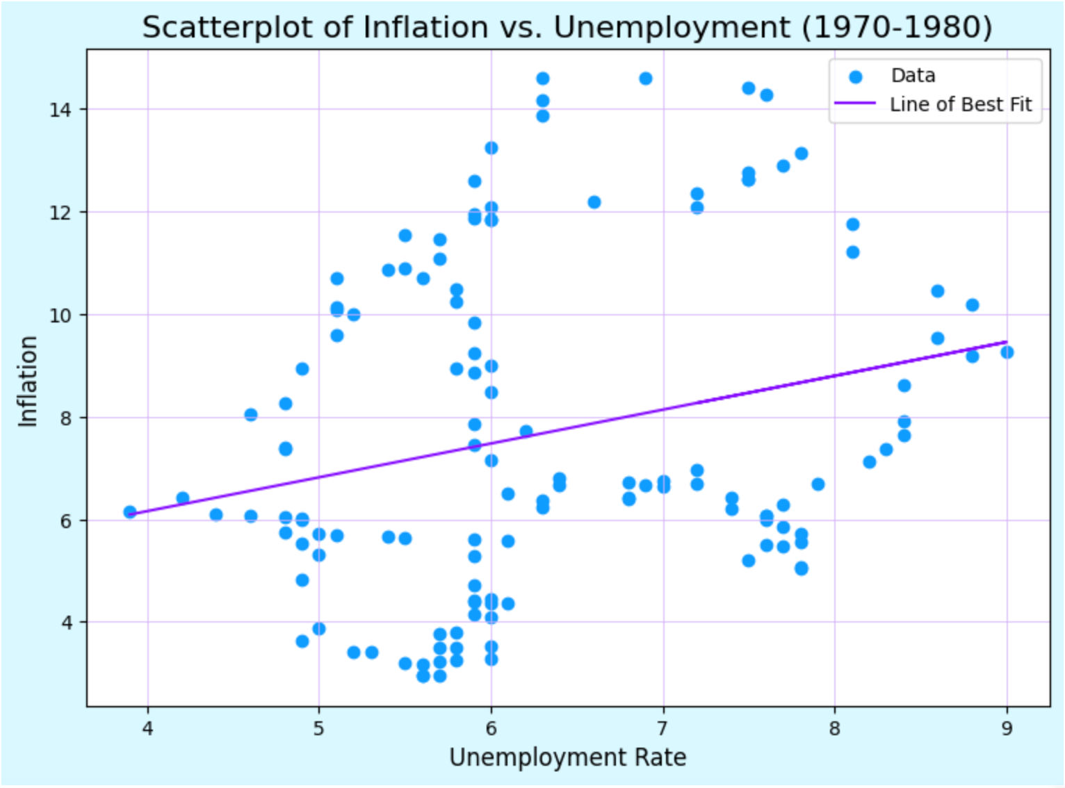
For example, if you were a macro investor in the 70s when the traditional Keynesian Phillips curve was widely believed (equation shown below) and you understood the role inflation expectations had in fueling inflation (second equation below), you could make significant money betting on continued inflation acceleration as expectations drifted upwards. Investors without this understanding would be using their knowledge of the recent relationship between the labor market and inflation (Figure 1) which proved inadequate for dealing with the new economic regime (Figure 2). In this case, your alpha was in discovering a new fundamental macro relationship.
Figure 1: Before the 70s, Unemployment and Inflation Were Negatively Correlated

Figure 2: Unemployment and Inflation Became Correlated in Response to Supply Shocks and Higher Inflation Expectations

Continuing with this general example, I’ve done research showing the traditional labor market vs. inflation relationship is tremendously misunderstood. The current dominant model is the New-Keynesian equation (shown above). This model has been horrible at predicting inflation and understanding how the labor market affects prices.
Those using the New-Keynesian model predicted the U.S. would experience rapid inflation in the post-2010s period and then failed to predict the surge in inflation during the post-pandemic era. The issue with the New-Keynesian Model is that it assumes a linear relationship between the labor market and inflation when the relationship is nonlinear. When unemployment is very low, employers must offer higher wages to attract additional labor, pushing their marginal cost up and increasing prices. However, when unemployment is high, workers are still reluctant to work for below-market wages, and thus marginal cost doesn’t fall significantly. It makes more sense to model labor market tightness rather than unemployment as well.
This is shown clearly in the data—there seems to be a strong relationship when there is an acute shortage of labor (more job openings than workers looking for work) and practically no relationship when the labor market is functioning normally (Figure 3).
Nonlinear inflation models outperform the best linear inflation models while offering a greater understanding of the underlying dynamics at play. In the 2010s, economists complained about a potential “flattening” of the Phillips Curve and then started to panic when the Phillips Curve was “steepening” in 2021. My nonlinear model determined the relationship was weakest when labor market tightness is roughly .7 and continues to strengthen the tighter the market gets. In Figure 4, I showed two notable examples of economists complaining about the “changing” labor-inflation dynamics despite no real change occurring for those who used optimal models. Those who understand this nonlinear relationship would have been better positioned to capitalize on higher inflation in the aftermath of the pandemic (Figure 5). This is an example of how understanding a fundamental macro relationship better than others can lead to alpha.
Figure 3: Significant Nonlinearities at Play Despite Dominant Models Showing a Linear Relationship
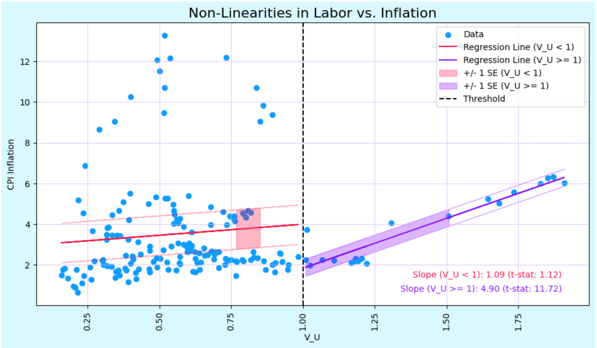
Figure 4: Those Using Linear Models Were Fooled by Path of Inflation Since 2008
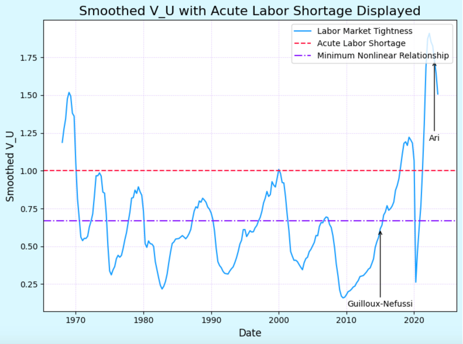
Figure 5: Acute Labor Shortage Contributed to Inflation Acceleration

The issue with this source of alpha is that it is temporary. Eventually, the market figures out these fundamental relationships. Investors talk, traders leave firms and spill secrets, and analysts gather enough data to exploit these opportunities. This alpha decays.
Alpha Decay in Factors
Perhaps I will devote a Sunday piece to this idea, but for now, I will only quickly touch on factor investing. Factor investing is the idea there are a few “factors” that offer excess returns. The most common factors are value, quality, and momentum. Each of these factors is said to have reasons for why they work—value works because of changes in multiples (they are priced so cheap and are disliked so much, that they can only be re-rated upwards). Value exploits behavioral biases:
“High-priced glamour stocks are more apt to experience unusually large negative price movements, usually after a string of negative news. The converse is true for value stocks. As a result, stocks with negative paradigms outperform stocks with positive paradigms because, when those paradigms are proven wrong, the stock prices move dramatically. These empirical truths have been widely validated
Those who try to predict fail, and the stocks of companies that are predicted to grow underperform the stocks of companies that are predicted not to grow. Growth is simply not predictable.26”
But, eventually, enough capital flows into factor funds and enough smart investors understand why the anomaly exists. Investors begin to overweight value, momentum, and quality and this erodes their relative returns. It’s a bit like the observer effect in quantum mechanics—when the market is observed, it gets understood and sources of excess returns disappear. Perhaps that is why value has done so poorly over the last fifteen years.
Macro relationships are always changing and I believe it is up to the discretionary investor to understand new dynamics as they appear. Regressions are likely far too slow-moving to understand trends in their infancy and ML models likely don’t have enough data points to truly discern what is signal and what is noise in the beginning. However, by understanding economic linkages better (and earlier), an astute macro analyst can discover new relationships as they emerge. Eventually, machines (and other investors) gather enough data to learn this linkage, the alpha dissipates, and the cycle repeats (Figure 6).
Figure 6: Profits in a Continuously Evolving Market

Alpha Source 2: Modeling Known Relationships Better Than Others
The second source of alpha is taking a known relationship and modeling one aspect of it better than others. For example, as inflation rises bond yields tend to rise. Firms that model inflation better than others can make excess returns trading bonds.
This source of alpha is generally a resources game. Those with greater access to resources (datasets, complex models, experts) will tend to outperform. But, there is an inherent limit to the ability to do this. Let’s look at the CPI report. Every month, the BLS releases its measurement of last month’s inflation rate. They do this by calculating a representative basket of goods and services and determining how these prices change over the course of a month. Much of the CPI is influenced by opaque and hard-to-forecast survey data:
“The CPI survey collects about 8,000 rental housing unit quotes each month to compute the indexes for the housing component. It uses price quotes for rent and homeowners' equivalent rent (an estimate of the implicit rent that owner occupants would have to pay if they were renting their homes) to compute estimates of price change. The housing sample is divided into six panels, with the housing units in each panel priced twice per year. Rents are collected by personal visit or phone.”
There is a level of inherent randomness to the outcome of this data. Understanding relative price trends can allow investors to get a rough estimate of what the CPI print will be, but it seems it is impossible to get a precise point estimate for inflation. It’s possible one’s model of inflation is superior to the BLS measure. However, the goal isn’t to predict inflation better than the BLS, it’s to predict what the CPI print will be! As more and more firms gather better datasets and push more resources toward predicting CPI prints, the market expectations will improve until the alpha from this strategy decays.
This type of alpha—forecasting known relationships better than others—is easier to do on short-term horizons than long-term horizons as there is greater variance in outcomes in the long term. There is also significantly more competition in the short run, making this alpha extremely hard to capture.
Now that we understand the sources of alpha in macro, we can begin to understand how regression models work—and where they can go wrong.
Regression Modeling
Harvesting Alpha Through Regressions
One popular way to exploit anomalies is through regression-based modeling. Using the first example from earlier, if you’re trying to predict inflation using labor market and inflation expectations data, how should you determine the relative weight to place on inflation expectations and labor market tightness? What happens if inflation expectations fall while the labor market tightens—do you predict inflation will rise or fall? I tend to like the principle of parsimony and thus prefer simple models to prevent overfitting. In this case, using an OLS or ridge regression appeals to me. Train your predicted equation (shown below) on past data and let the model determine the values for your coefficients. Then, plug in current data and let that determine your forecasts.
For the second source of macro alpha—measuring a known relationship better than others—regressions also allow investors to understand how to weigh different data points. In determining the CPI weight, many funds have a regression with many different variables (one for gas prices, another for labor market tightness, another for expectations, and so on) that helps them predict inflation more precisely. It is rather impossible to incorporate the vast swath of data involved in inflation calculations solely in your head. Thus, investors tend to rely on regressions.
Regressions are incredibly popular in macro modeling. Regression modeling provides a way to weigh the relative importance of different data points and reduces the ability to overfit by imposing a somewhat rigid structure on the investor.
Vulnerability to Regime Changes
Regressions are great, but they suffer from a huge vulnerability—a lack of agility in adapting to regime changes. There are periods where some factors work more than others, periods where inflation prints matter, and those when CPI days are non-events. Often, these changes in macro relationships follow a big event—Fed meetings were huge in the aftermath of the pandemic (will they increase QE?). Other times, they are in response to changes in a specific variable (CPI prints matter more when inflation is high than when it hovers near 2%). Regressions do poorly when adapting to regime changes because they need lots of data points to change. Every day that passes in a new regime enables the regression to improve—but it will underperform in the short term as it attempts to “learn” the new environment.
It is precisely during economic regime changes when sources of alpha are most plentiful, yet difficult to find. When previous linkages break down and new ones are formed, it takes time to discover them. When the financial system collapsed in 2008, the Fed took on a new and bigger role in markets. Investors could get excess returns by understanding how QE would affect markets (1. discovering new linkages) or by predicting the path of the Fed balance sheet (2. modeling known relationships better). This alpha is inherently difficult—because a new regime is starting there are few data points and regression-based models are of little use.
Solutions to the “New Regime Issue”
1. Rise of Discretionary Investors
Much has been said about the end of discretionary macro and the pivot towards systematic macro. While I understand and often agree with the desire to systematize certain trading rules, I do not think discretionary macro is dead. I think there are certain periods in which systematic outperforms discretionary and others where discretionary triumphs. I believe discretionary macro tends to outperform at the beginning of regime changes while systematic macro outperforms once a new regime is established and there are enough data points to make models more efficient.
Discretionary investors who understand new macro relationships can outperform regression-based models in the short run, harvesting excess profits as they wait for these models to understand the new environment. At the beginning of a regime change, the future-focused discretionary investor is facing off against a backward-looking regression-based model. The model has given weights to certain data points based on the recent past. The discretionary investor is far more flexible (both an advantage and a burden!) and can understand that what once mattered may no longer matter (and what once was overlooked may now be important).
I’ve made it seem extremely simple for the discretionary trader—it’s not! It’s very hard to understand how the economy will change in response to a new development. Imagine how difficult it would have been to predict the impacts of QE on markets and the wider economy when it first began in the U.S.? It requires a curious investor, a creative thinker, and a student of economic history to make the connections necessary to foresee the future of markets.
2. Weighted Regressions
The issue with regressions is they often take significant time to adapt to regime changes. If I have a regression model that was trained on the past ten years, the data point from yesterday matters as much as the data point from nine years ago. This makes learning a slow process as it requires a lot of data to “unlearn” old, obsolete relationships. Let’s visualize this.
First, let’s look at the scatterplot between inflation and unemployment from 1950-1980 (Figure 7). Throughout the entire period, the relationship between unemployment and inflation was positive. However, this total graph obscures the nuances of the picture.
Figure 7: Positive Relationship Between Unemployment and Inflation from 1950-1980.

From 1950-1970, the relationship was strongly negative (Figure 8). While not prevalent at the time, regression-based models would have assumed the 1970s would continue in this pattern. Lower unemployment rates would predict higher inflation rates and higher unemployment rates would lead to lower inflation. However, that’s not what happened! In the 1970s, the relationship flipped (Figure 9). Because of the way regression modeling works, the vast amount of data between 1950-1970 with a negative relationship between unemployment and inflation made the model extremely slow at understanding the new positive relationship between the two.1 It wasn’t until around 1975 that the regression model would show a positive relationship between unemployment and inflation!
Figure 8: Before 1970, Inflation and Unemployment Were Negatively Related

Figure 9: Relationship Between Unemployment and Inflation Turned Strongly Positive in the 1970s
Ok, so how to fix this? We know when we are entering a new economic regime, regressions often take too long to learn so we need to speed up that process. I spent time developing two ways to improve regressions with the second being an improvement of the first.
First, one can use time-weighted regressions. The idea of these regressions is data in the recent past should matter more than data in the distant past. Why should data from 2009 be counted the same as data from yesterday? By doing this, you speed up the learning process of the regression. My preferred way of doing this is to decay the weights of data points by some equal amount pertaining to some half-life (the exact optimal half-life likely depends on the series and shouldn’t truly be optimized to prevent overfitting) and keep a baseline asymptotic weight. For example, yesterday’s data point may count as “2” and every day before may be weighted in a similar manner as the equation below. So, the point 100 days ago has a weight of around 1.37.
[Side note: Perhaps I will devote more time to this idea, but it’s possible if one believes a certain historical period could explain returns well for the current period that one can weigh some time periods as more impactful than other periods. However, this has massive potential for overfitting and I caution against it].
A more advanced version of one is a variance-weighted regression. I’ve previously explored the idea of variance time and variance as information here. The higher the variance in markets, the more information is being digested by them. Variance exists precisely because new information is being incorporated into markets. Not all time is weighted equally in markets—times with higher volatility are periods when more information is digested. Moreover, higher variance periods tend to precede new regimes—that’s why there is volatility! Perhaps then, when weighting our regressions, we should not count each day as equal. Decay should not be by calendar day but determined by variance. The weight of a data point decays by the sum of the variance that has occurred since that day, not the sum of the days since then! By doing so, we speed up the regression’s learning in a more optimal way—enabling our model to adapt to regime changes, capture alpha quicker, and relatively “unlearn” obsolete relationships.
3. Fund Structure
I believe funds that optimally balance both discretionary and systematic strategies are best positioned to earn excess returns throughout the market cycle. Discretionary traders should outperform at the beginning of new regimes while systematic algorithms will grab the baton once the regime is fully in motion. By using weighted models (preferably variance-weighted), systematic models can begin to outperform earlier and more strongly than they otherwise would.
Funds with open communication between their discretionary and systematic sides can optimally determine when to size up on systematic bets and when to weight more towards the discretionary side. Moreover, discretionary traders may be able to help systematic investors determine when and where their models may be wrong. By working together, they can improve these models and allow them to profit in new market environments. Moreover, traders who understand how certain models are structured can take advantage of antiquated regressions and position themselves on the other side of their trades—profiting from their ignorance.
Conclusion
There are generally two main ways to capture alpha in macro—discovering a new economic linkage and measuring a known relationship better than others. Regression-based models excel at performing each of these tasks once we have settled into a stable economic environment and enough data exists to exploit anomalies. However, at the cusp of regime changes, when economic relationships are in flux, regression models are likely to make significant mistakes. By understanding the dynamics of economic linkages in the new environment before enough data allows models to profit, discretionary investors can harvest significant alpha. Moreover, regression models should speed up their learning process during the beginning of regime changes by using time-weighted or variance-weighted regressions. Lastly, funds with a good balance between discretionary and systematic trading will likely earn stable returns throughout the market cycle. Collaboration between these two sets of strategies should improve returns overall. More risk should be allocated to discretionary investors at the beginning of a new regime while more risk should be given to systematic investors once we settle into a new regime.
Extra:
Here are a few things I read/did/researched this week that I found interesting.
Kelly Betting and Skew
I found this paper rather interesting. The paper explores the Kelly Criterion and the potential pitfalls with it. The Kelly Criterion is an elegant solution to determine bet sizing. For example, say you have $100 and someone offers you a coin flip bet: if the coin lands heads, you get $200 (wealth = $300) and if it lands tails, you lose your $100. Expected value states you should take this bet (50% * 300 + 50% * 0) = $150 > $100. The Kelly Criterion focuses on the geometric mean and notes, correctly that the gamble is a long-run failure (if you continuously take +200%, -100% bets you are sure to lose everything!
However, this paper shows the Kelly Criterion ignores hire-order moments of a distribution. It bets significantly too much with negatively skewed bets. Thus, one must adjust for the skewness of the distribution as shown here. I think Kelly math is rather fascinating so I enjoyed this short paper.
Fiscal Dominance and IORB
I previously wrote a bit about fiscal dominance here. I find the topic extremely intellectually stimulating, but so far, I think it is more narrative than science. This paper explored the implications of continued high deficits and future entitlement spending. Calomiris believes one of the ways out of the debt trap is if the Fed forces banks to hold a greater amount of reserves at the Fed and lowers IORB to 0%. This would be a massive tax on banks but would lower the inflationary burden on the rest of the economy. Given that banks are rather unpopular, this could be the public’s favored solution to a difficult problem.
The Office
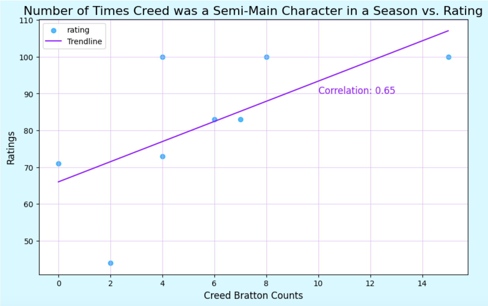
For a Data Science project this week I had to scrape The Office fandom page and gather a bunch of data on individual episodes. I put together this ridiculous chart showing the correlation between the number of episodes in a season where Creed Bratton was a major character and the Rotten Tomatoes rating of the season (Figure 10). I thought any Office fans who read the Substack would enjoy this.
Figure 10: Reviewers Seemed to Love Creed Bratton (Or Correlation, not Causation?)
LSE Tennis Wins Southeastern Cup
I’ve been playing on the LSE Varsity tennis team this school year and we finished up our season on Wednesday winning the U.K. Southeastern Cup against Surrey. We won 5-1 and played very well (Figure 11). It was a super fun season and I assume it was LSE’s best in recent memory. We went undefeated in team play with 14 wins. I greatly enjoyed playing again after having retired from tennis during my freshman year. This may be the end of my competitive athletic career, but I’m glad to have finished on a high note.
Figure 11: LSE Battling During a 5-1 Victory in the Cup Final

Thank You!
Thank you for reading until the end. I’m very grateful for the ability to share my thoughts on markets, macro, and anything else I’ve been interested in. I spend a lot of time formulating ideas and thinking about this Substack. I’d love to continue talking with readers—reach out and share this with anyone who may be interested! I hope you have a great weekend.
-Eli
Of course, one could argue the ceteris paribus relationship remained negative. However, that is not the point of this—the point is to explore how regression-based models can be extremely slow at adapting to new regimes. Additionally, solving the “ceteris paribus” question requires knowing the variables to control for which isn’t a given in a dynamic environment. In fact, finding these variables is a form of alpha (discovering a new relationship).